Is state really bad?

Prologue

Actually this post was being written in March, when some facts referred in the body of the article actually happened. I am resuming the post today, after months of extensive (and rather unbloggable) work.

Intro

Stateful programming is somewhat the default strategy in the industry nowadays and it has been in the last 60 years. If we consider the 10 more widespread languages in the tiobe index (a statistic is worth another), they are all imperative languages strongly based on stateful programming. This month Lisp is has enormously improved (Land of Lisp anyone?), but even if we would consider Common Lisp and Scheme together, it would not go in the first 10 positions (even if just for a few points).

The Haskell case

In fact, in the last years we have witness an increase of interest in functional languages. As far as I remember, about 5 years ago there was a lot of hype about Haskell (which was in its 30's or something like that). It was related, as far as I remember, in a famous user-friendly linux distro having written some tools in Haskell and in the Darcs project. Darcs has almost disappeared with Git (Perl+C) and Mercurial/Bazaar (Python, Python+C) sharing the market of distributed versioning tools.

The case is rather interesting: Darcs was built with a very strong "theory" behind, the algebra of patches. The problem is that the merge process is still exponential in the worse case and that it is rather buggy. It is interesting that the software is both slow and bug ridden. It is tempting to infer something about Haskell, at least to counter the hypothesis that pure functional programming makes it relatively easy to write bug-free programs. Perhaps this should be taken into account the next time someone looks down on setf. Well, I do like Haskell, just not as much as I love Lisp.

The last thing I would like to mention is that I like the idea to insulate imperative code from functional/algorithmic code (but this is something I suggest with every language). However being forced to do that is not necessarily a good idea. In fact, it makes Haskell quite harder to pick up and has the paradoxical effect that if you are a developer good enough to code in Haskell, you probably already know how to separate side-effected code from side-effect free code. Besides, although I like purity (to some extent), I'm not sure whether state monads should be considered stateless. I mean, a state monad implements state in a nice functional construct, mathematically sound and pure. In fact they are almost seen as an executable transaltion of the declarative semantics of a stateful program. Consequently, I'm not sure whether frequent use of state monads is really an improvement over carefully used stateful programming.

In other words, although I admit my limited experience of Haskell in real world projects, I believe that if we think functionally the code is going to be clear (but it will be as clear in Haskell as in Lisp). On the other hand, if we think in a heavily stateful way, our code may be less clear in Lisp and quite messy in Haskell, where we would implement our (wrong) thinking having state monads pop out everywhere. Feel free to correct me, possibly with real experience and examples.

Erlang and Clojure

Erlang is different from Haskell in that functional stateless programming is required for practical purposes. In order to allow shared-nothing process based architecture (and the actor model), state is essentially banned. Of course, there are solutions which bring back state (ETS, DTS, plus various libraries such as mnesia). It is worth noting that this kind of state is generally different from usual imperative state.

In imperative languages everything is stateful by default. On the other hand, in this case, we basically have only "db like" solutions. This does not encourage real stateful programming, and in fact, usual Erlang programs are pretty much state free. The essential different is that they are not side-effect free.

Being state free and side effect free are two very different things. Having no side effects is pure functional programming. And is extremely hard to do. In fact, it would not even made sense in a programming language built around the idea of passing messages between processes. If you send a message, you are not side-effect free anymore.

Somewhat in the same sense, Clojure is stateless but not side effect free. Most clojure coding is performed without explicit state change and there are a few explicit ways to deal with state. This is done in transactional way, so that essentially state change is allowed if explicitly required. State change should not mingled with stuff which has effect outside the clojure process. You can "unset" a variable and recover the old value, but you cannot unsend a message.

At the moment I feel that I can easily tolerate (and like) the kind of state change insulation provided by clojure and the pragmatics of avoiding side-effected stuff for as long as possible typical of all functional languages. On the other hand, I find really hard to accept absolute stateless-ness.

Lisp and Languages with FOFs

On the other hand of the spectrum of "functional languages" we have Common Lisp and the various freedom languages where functions are first order objects (Python, Ruby, ...), with Scheme leaning a bit more towards the functional side. Technically speaking Python is not even a functional language. Surely it is not stateless (but Lisp is neither). In fact, in Python recursion is frowned in favor of iteration (but iteration is often built around generators, which are an user-friendly/dumbed-down[0] instance of anamorphism -- unfold --, which is strongly functionally flavored). On the other hand, some call Ruby the Matz-Lisp.
In these languages there is no explicit restriction towards stateful programming. This means that usual algorithms and way of thinking are easy to implement (especially in Lisp, both very functional and very stateful algorithms are easy to implement). On the other hand, restriction of state change is left to the sense of the programmer (which not always is a good thing, but I don't really like languages which tell me exactly what to do... they just have to make the better way obvious -- I'm not Dutch, sorry --).
To be sincere, there are just things that are so much easier in stateful programming than in stateless programming. And for other stuff the converse applies. Consequently, the language should not force me too much towards one style or the other. Moreover, stateless-only languages tend to be harder to pick up for beginners (on the other hand Python and Ruby are extremely easy to start with and I believe that scheme is a wonderful first language for computer scientists). Eventually, stuff like GUIs are really hard to implement in fully stateless settings (clojure essentially relies on Java underlying classes, and I actually have never used Erlang for guis -- not that I am a strong GUI developer --).

On performance

One of the consequences is that lots of algorithms, data structures and ideas are just developed with stateful programming in mind. This is the reason books suck as Okasaki's Purely Functional Data Structures have been written: just to bridge the gap between mainstream stateful programming and functional reasoning.

Unfortunately many algorithms have been created with imperative languages in mind, and the data structures supporting the algorithms strongly reflect the imperative setting. Implementing such algorithms in functional settings is usually inefficient to say the least. Much theory (and not only the practice) is built around state change. The Art of Computer Programming uses a pseudo assembly language which essentially manipulates a Von Neumann machine.

Something as easy as "modify an array" may be a source of inefficiency in many languages. E.g., clojure provides transients just to make it easier to express such operations. On the other hand functional languages have usually some troubles in providing a data structure that is immutable, offers O(1) random element access and allows element modifications without copying the whole data structure.

Books

"Purely Functional Data Structures" (Chris Okasaki)

"Art of Computer Programming, The, Volumes 1-3 Boxed Set (3rd Edition) (Vol 1-3)" (Donald E. Knuth)

Notes

[0] depends on whether you are a python or a scheme programmer: python programmers usually say user-friendly

Combinatory Logic in Lisp

Many year ago, I was introduced to a formalism called "combinatory language". I quite fell in love with it, but that my personal taste. Combinatory logic, according to Wikipedia, was originally introduced as a notation to remove variables from logic. However, in the presentation I'm familiar with variables are used [1]. In fact, I have seen it a computation model: combinatory language is proved equivalent to lambda calculus (trivial) and as such it is also a computation model (and a possible foundation for functional programming).

The fundamental units are combinators, that is to say elementary (higher order) functions. The result of the computation comes from function application (but the elementary functions are so simple that it is possible to see implement the evaluation just as a simple rewrite system). In fact, just two combinators are needed S and K (definition follows). Usually the I combinator is defined as well, but that can be defined in terms of K and S, so it is not "primitive".

Quite interestingly, it is possible to use combinatory logic to define regular first order logic. So it can be a model for mathematics as well... and some rather important (and difficult to prove) theorems in logic are rather elementary and easy results in combinatory logic. But well... to the metal.

Let us have an infinite sequence of variables (lowercase) and a finite or infinite sequence of constants (uppercase), including the three fundamental combinators I, K, S.  Variables and constants are atoms. The definition of combinatory term is as follows:

1. Every atom is a combinatory term
2. If X and Y are combinatory terms, (XY) is a combinatory term as well
   

A combinator is a combinatory term whose atoms are only S, K, I. Variables are disjoint from constants.

Since combinatory logic is very "operative" we define the fundamental computation tool, which is the weak reduction.

• IX -> X
  
• KXY -> X
  
• SXYZ -> XZ(YZ)
• X -> X
  

where the parentheses have the usual meaning (that is to say xzu where u is the result of evaluating yz). Right now I don't want to introduce axioms regarding variables. Now I rewrite the combinators as "usual functions" to clarify what they really do:

• I(f) = f
• (K(a))(x) = a
• (S(f, g))(x) = f(x, g(x))
• (B(f, g))(x) = f(g(x))

The B combinator is not fundamental, and can be easily defined as S(KS)K. So now we have a pretty clear idea of what combinators are. I corresponds to the identity function. K is "like" a function returning a constant whatever arguments we pass. In fact K is a "function" which given something yields the function always returning that something. B is a function composition operator. S is a bit harder to understand (but wait to see the Y combintor! ;) ),

My first significant lisp program years ago was the implementation (in lisp) of the the basic computable functions (primitive recursive and mu operator, IIRC what I did). I thought that a nice example of another lisp program could be implementing the combinators in Lisp. After doing some more theory (e.g., we haven't yet stated how to "compute" programs or represent numbers), we can go for the implementation.



References

1. R. Hindley, B. Lercher, J. P. Seldin, Introduction to combinatory logic (CUP Archive, 1972), p. 170

Combinators, Combinatory Logic, Logic, Maths, Lisp, Functional Programming, Foundation

Powered by ScribeFire.

Geometry/graphics algorithms: segment intersection

With modern gaming libraries dealing with most geometric/graphics issues, it is probably possible to create simple (and not so simple) games without a clue on the basics of computational geometry. However, the elementary algorithms are really so simple that it is worth to keep them in mind nonetheless.
First, I will briefly review some mathematical concepts we will be using, then I will present the algorithms. In this post I will present algorithms to find if two consecutive segments represent a left or a right turn and to discover whether two segments intersect.
The segment intersection is probably the single most important operation: for example it can be used as a building block to detect collisions in a 2D-game and can be generalized to work with 3D games as well.

Magic of the cross product

For those who thought that they belonged to somewhere else during the geometry classes (or who profoundly hated trigonometry) this will be short. Moreover, we won't use sin and cos since they are extremely slow operations. Nor will we use divisions (as they are both slow and yield to potentially badly conditioned algorithms).

Let A and B two vectors, that is to say two segments with the origin in the origin of the system (0, 0). Their cross product A x B is defined as:

Physics (and mathematicians) would say that A x B is a vector perpendicular to both A and B (thus not contained in the considered 2D plane) according to the right hand rule and with magnitude |x_Ay_B-x_By_A|. However, we are only interested in the sign:

• If the cross-product is negative, then A is counterclockwise from B
• If the cross-product is 0, then A and B are collinear
• If the cross-product is positive, then A is clockwise from B

Our second step is to consider pairs of segments with one end in common. Let s=CA and t=CB (CA and CB should have a bar above, but I can’t do that for typographical reasons) be the segments, where A=( x’s, y’s), B=( x’t, y’t) and C=(x, y).
We know how to compute whether the segment CA is clockwise from the segment CB, that is to say:
As a consequence:

• If the cross-product is negative, then CA is counterclockwise from CB
• If the cross-product is 0, then CA and CB are collinear
• If the cross-product is positive, then CA is clockwise from CB

Turn left or turn right?

Now, given the consecutive segments AB and BC, we want to find out whether going into BC is a left or a right turn. A simple schema clarifies the thing.

Essentially we can compute the cross product ACxAB in order to discover if BC is a left or right turn with respect to AB. This is a very important building block to compute the segment intersection.
We notice how we did not use sin, cos or divisions. We have simply a bunch of multiplications, sums and subtractions. It is even likely that some architecture can perform the determinant of a matrix with a single operation.

Segment intersection

At this stage, we can introduce the code to compute the segment intersection. First I present the function computing the direction between two given segments. Considering that we do not want to make this functions dependent from the specific representation of segments, we just let it take the points A, B and C.
The function uses only multiplications, additions and other elementary inexpensive operations (no divisions, no cos or sin). The basic idea is using the simple function we defined in the last section and eventually deal with the special case when one segment end lies on the other segment.

So, the function is:

def direction(origin, first, second):
    return cross_product(second-origin, first-origin)

provided that we represented points like that:

import collections

def cross_product(lhs, rhs):
    return lhs.x * rhs.y - lhs.y * rhs.x

class Point(collections.namedtuple('Point', 'x y')):
    def __add__(self, other):
        return Point(self.x+other.x, self.y+other.y)

    def __sub__(self, other):
        return Point(self.x-other.x, self.y-other.y)

def direction(origin, first, second):
    return cross_product(second-origin, first-origin)

Notice the use of named tuples here. We have efficiency of tuples and ease of use of regular classes. But this is another story. Then, we have the real thing:

def does_intersect(first_start, first_end, second_start, second_end):
    direction_1 = direction(second_start, second_end, first_start)
    direction_2 = direction(second_start, second_end, first_end)
    direction_3 = direction(first_start, first_end, second_start)
    direction_4 = direction(first_start, first_end, second_end)

    if (direction_1 * direction_2 < 0
        and direction_3 * direction_4 < 0):
        return True
    elif direction_1 == 0 and on_segment(second_start, second_end, first_start):
        return True
    elif direction_2 == 0 and on_segment(second_start, second_end, first_end):
        return True
    elif direction_3 == 0 and on_segment(first_start, first_end, second_start):
        return True
    elif direction_4 == 0 and on_segment(first_start, first_end, second_end):
        return True
    else:
        return False

What do we mean? direction_1 tells us "on which side" the start of the first segment is with respect to the second segment. On the other hand, direction_2 tells us on which side the second segment end lies. If both points are on the same side (they are both left turns or right turns), then the two segments do not intersect. But if the extremes of the first segment are on different side of the second segment and the extremes of the second segment are on different sides of the first segment, then it means that the two segments must have an intersection. The rest of the procedure deals with collinear segments: in this case some extreme of one segment must lie on the other segment. The last procedure is:

def on_segment(origin, first, second):
    if (min(origin.x, first.x) <= second.x <= max(origin.x, first.x)
        and min(origin.y, first.y) <= second.y <= may(origin.y, first.y)):
        return True
    return False 

Segment Intersection, Computational Geometry, Python, Algorithms, Geometric Algorithms, Games, Gaming Algorithms

Java Collections sorting: copy, copy & copy in every sense!

This morning I was hacking into OpenJDK some implementation details. Curiosity, perhaps.

After the announcement that Java is going to use timsort for generic sorting (which is a very good piece of news).
By the way, this is an actual implementation. I'm also wondering why these things are mostly ignored in Algorithm courses, but this is another story.

So... I checked the actual implementation. I had to download the OpenJDK source, as apparently on OS X IntelliJ does not auto-show implementation of base classes when I "jump to implementation". Anyway... the implementation of sorting is basically in Arrays.java.

I want to point out the funny comment relative to sort1 (which is the private function which actually does the job for non floating point stuff):
    /*
     * The code for each of the seven primitive types is largely identical.
     * C'est la vie.
     */

which really saved the day... Yes... it is almost cut and paste for the primitive types (char, int, byte, etc). I was amazed... it is 2010, we have generics but, as primitive types are not objects we have to actually write it 7 times. As a side note, code is recursive quicksort variant.

Ok, nice. You have implementation constraints and you have to cope with that. Yes... C++ templates perfectly solve this crap. But then, there is another very funny discovery (well, in fact I have known this for quite a few time). But that is not the only (technically) unnecessary copy which happen(ed|s) when dealing with sorting in Java; this is the sort function in Collections.java

public static <T extends Comparable<? super T>> void sort(List<T> list) {
Object[] a = list.toArray();
Arrays.sort(a);
ListIterator<T> i = list.listIterator();
for (int j=0; j<a.length; j++) {
i.next();
i.set((T)a[j]);
}
}

Wow! It is clear what it does? For every collection you sort, a copy is made. To be honest, the documentation states this clearly:

This implementation dumps the specified list into an array, sorts
the array, and iterates over the list resetting each element
from the corresponding position in the array. This avoids the
n^2 log(n) performance that would result from attempting
to sort a linked list in place.

Nice! Very nice... this means that the default sort function may be unnecessarily slow. Unless you use arrays (but using arrays in place of collections is considered a bad practice). Moreover, Collection is an interface: its implementation may be such that a full copy into main memory is not feasible. BTW, I should double check because the comments in Arrays.sort state that the algorithm is a modified quicksort, not a modified mergesort.

Oh... nice! Tomorrow I am discussing other methods in Arrays and Collections.

Anagrams: fast python algorithm

So in this post I showed how the trivial algorithm to compute anagrams is stupid (and consequently slow) beyond hope. On the other hand I promised a nice algorithm to do that. In fact, it is just a matter of pre-processing the data. The idea is to compute a key which is unique to all the words which have the very same letters and then group all the words with the same key. One of the simplest keys could be a bag of the letters (if your language supports bags -- or multi-sets --). Python sets have unique keys, so they are not a good candidate. However a "sorted" variant of the word has the right properties. Every word with the same letters (which is the definition of palindrome) yields the same string if we sort its letters. A good structure is a dictionary with this key as key and a list of strings as value. When we find a string with a previously found key, we add it to the list of strings, otherwise we generate a new list. This is the very popular setdefault idiom:

d.setdefault(key, []).append(w)

The key for a word of length n is computed in O(n log n), insertion in the dictionary is O(1) (get the key is O(1) in average and append to the list is O(1)). So the algorithm uses rather efficient elementary operations. At this point "general" questions on the processed wordlist can be answered in O(M) if M is the number of the words (e.g., longest anagram, word with most anagrams). Simply getting the anagrams of a given word is an O(n log n) operation. We are not using an excessive amount of memory. We basically have an hash-table and some "pointers" to the original words. And now the code:

class Anagrams(object):
    def __init__(self, dictionary):
        self.dictionary = dictionary
        self.indexed_words = {}
        self.preprocess()

    def make_key(self, word):
        sorted_word = list(word)
        sorted_word.sort()
        return tuple(sorted_word)

    def preprocess(self):
        for word in self.dictionary:
            key = self.make_key(word)
            self.indexed_words.setdefault(key, []).append(word)

    def anagram(self, word):
        key = self.make_key(word)
        return tuple(self.indexed_words[key])

    def anagrams(self):
        return [anagrams for key, anagrams in self.indexed_words.iteritems()
                if len(anagrams) > 1]

As a matter of fact, if we extend the corpus of words, the required time increases. In fact, using the dictionary from here it took 4 whole seconds. Which is nonetheless a lot less time than some million of years. I did not use that dictionary because it contains lots of misspells which can have sense when computing Levenshtein distances, but are quite a PITA if we compute anagrams (we don't want non existing words to popup as solutions).

Technorati Tags: Efficiency, Optimization, Python, Algorithms, Anagram

Anagrams and (brains vs. cpu)

In AI there is a vast category of algorithms which follow a (blind) generate and test strategy. They essentially "generate" the solutions (as a whole or step by step) and then test if the solution complies with an acceptance function. Unfortunately, this simple strategy is usually ineffective. The cost is often exponential in the size of the input and since there is no "intelligence" all solutions (even dumb ones) are explored). In AI it is customary to use smarter search techniques (A*) or to "change" the problem so that even smarter solutions are viable. An apparently unrelated example, is "finding the anagrams of a word". The trivial (and generate and test) solution is:

1. [generate]: try all the permutations of the word
2. [test]: check if the word is in the dictionary

and this strategy also shares the very same problems of the other generate and test strategies. All the permutation of a k characters word are k! = k(k-1)(k-1)...2. It is customary to see algorithms like:

def yield_anagrams(dictionary, word):
return [word for word in
(''.join(candidate) for candidate in it.permutations(word))
if word in dictionary]

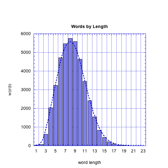
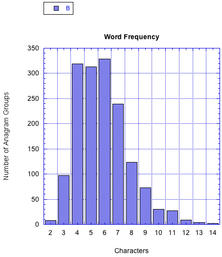
which in other languages are even longer and less attractive. This approach is rather tempting for very small words. I got some interesting wordlists from here. As a good starting point I used the 12Dict list and in particular the 2of12.txt file. More info on the lists can be found in the ReadMes. In the rest of the post we are going to work with that dictionary. This graph shows the distribution of word lengths: This other graph shows how many groups of words with the same anagram we have by word length: For those preferring tabular data:

Size of the word	Number of groups
2	8
3	97
4	319
5	313
6	329
7	239
8	124
9	73
10	30
11	27
12	9
13	4
14	2

As we can see, the longest words with anagrams are 14 characters long. Even though most anagrams are very short word, our algorithm should work reasonably well with every input. The code I showed cannot. For example, let us consider the time required to compute the anagrams of words of increasing size:

scoreless	9	0,174
praetorian	10	1,828
rationalize	11	21,03
indiscreetly	12	269,0

In the first graph, we both axes are linear. If we do not believe me when I say that the growth is exponential, then look at this other graph: here the y axis is in logarithmic scale. Exponential means that if you simply change the implementation or the implementation language, things are going to blow up once again a couple of steps later. So, let us sum up: we have 41238 words. Of these words, 5644 have 12 or more characters. If we suppose that anagrams for words longer than 12 character cost exactly as anagrams for words 12 characters long, the whole process is going to take 1518236 seconds, that is to say more than 17 days. In fact, the whole process is going to be far more expensive. I have a full table (excel -- here you may want to download the file --, csv) with times estimated using the formula derived from our 4 values. Of course, this is not extremely precise, but the sheer magnitude of the computed values should make the point clear. To compute all the anagrams for all the words up to size 11 (included) it takes one day. If you want to reach size 13 it is going to take one year. However, it is still a long way to process all the words... for example, in order to discover that our dictionary words with anagrams of length 15, our program is going to run for more than 38 years. The conclusion that no words longer than 14 has an anagram (according to our dictionary) takes more than 4000000 years. Of course, I did not wait all that time to gather these results... tomorrow I am showing a smarter strategy which drops the required time from 4000000 years to 0.16 seconds.

Technorati Tags: Efficiency, Optimization, Python, Algorithms, Anagram

How much do you cost me?

Introduction

Study of algorithms and data structures is a major field in computer science. Efficiently representing and processing data has been of paramount importance since the early days of computing. Many problems are simply not accessible without proper study, since the computational complexity used to overwhelm older machines.

Today, we have powerful machines. Tomorrow, we will have more powerful and “more parallel” machines. One day, our computers will surpass the computing power of our own brain. However, no matters how fast the computer it is, there are always problems which are too hard, too expensive and, in short, intractable.

Essentially, the cost of the algorithm depends from the size of its input. For example, searching for an element in a list intuitively takes time proportional to the number of elements: after all, we don’t know where it is, we have to start somewhere and the element could be at the other end of the list.

In this case we say that the worst case is exactly A∙N, if A is the cost of comparing two elements and N is the length of the list. The average case is “only” A∙(N/2) since “in average” the element will be found after examining only half of the elements. Intuitively, the probability the element is the last one, is equal to the probability it is the first one, and so one. Computing average case cost is usually harder than worst case cost, because involves probability and random variables.

Landau notation and estimates

The computational cost of algorithms is usually represented in a unified notation (called Landau notation, from the name of the famous mathematician who introduced the notation in the field of calculus). Essentially, we don’t care about the multiplicative constants in the costs (e.g., A, “the cost of comparing two elements”) as long as they are, well… constants. We usually say that an looking for an element in a list costs O(N), which means that the time is proportional to the size of the list itself.

Most of the times, computing the cost of an algorithm is rather straightforward. Considering a strictly imperative setting, you essentially estimate the number of times you run the body of a loop. For example, let us consider
the following code:

M = {}
n = 4

for i in xrange(0, n):
    for j in xrange(0, i):
        M[i,j] = M[j,i] = i + j

print M

It is rather easy to see that if A is the cost of M[i,j] = M[j,i] = i + j, the whole thing costs (using presumed Gauss's formula):

That is to say it's O(N^2). A (correct) but coarse argument is that the internal loop runs i times, and i is at most n. So in the worse case it is n. The upper bound is used as an estimate n*n (again O(n*n)).

Things are not always that easy: sometimes the worse case is completely uninteresting. E.g., the most widely used simplex algorithm[0] has an exponential worse case cost. Exponential means that it essentially sucks. 2^1000 is a huge[1] number and 1000 is not an extremely huge input size. In pratice, the simplex algorithm is used, since the average complexity is polynomial. There is still active research on the estimation of the complexity of that algorithm.

The Master Theorem

A large class of algorithms are called "divide et impera"; a typical example is mergesort[2]. Here a trivial python implementation is given:

def merge_sort(L):
    if len(L) <= 1:
        return L
    else:
        middle = len(L) / 2
        left = merge_sort(L[:middle])
        right = merge_sort(L[middle:])
        return merge(left, right)

def merge(left, right):
    i = j = 0
    max_i = len(left)
    max_j = len(right)
    sorted_ = []
    while i < max_i and j < max_j:
        if left[i] < right[j]:
            sorted_.append(left[i])
            i += 1
        else:
            sorted_.append(right[j])
            j += 1
    if i < max_i:
        sorted_.extend(left[i:])
    else:
        sorted_.extend(right[j:])
    return sorted_

Of course, no Python user would use such functions. They use recursion instead of iteration, they are not particularly efficient, the "Timsort"[3] implemented in the Python library is far more efficient both algorithmically and code-wise. Algorithm books tell us that merge-sort has worse and average case O(N log N). As with most divide et impera algorithms, the result can be proved with ad hoc demostrations. However, I found extremely useful using the so-called master theorem[4]. This is essentially a swiss-knife result that gives us the complexity of an algorithm given the way the data is "divided" and "recomposed" (to rule, of course!). The complexity of the algorithm on an input of size n is T(n). f(n) is the cost done outside the recursive calls (e.g., the time needed to decompose and put together the data); a is the number of subproblems in the recursion and n/b is the size of the input of the subproblems. For example, in merge-sort a = 2 and b = 2. f(n) is proportional to the size of the input vector. The master theorem states that if:

1. 
   
2. 
3. 
   

The big theta notation essentially says that the specified bound is asymptotically both a lower and an upper bound. The big omega means that the specified bound is a lower bound.

Notes

[0] http://en.wikipedia.org/wiki/Simplex_algorithm
[1] 10715086071862673209484250490600018105614048117055336074437503883703510511249361224931983788156958581275946729175531468251871452856923140435984577574698574803934567774824230985421074605062371141877954182153046474983581941267398767559165543946077062914571196477686542167660429831652624386837205668069376
[2] http://en.wikipedia.org/wiki/Merge_sort [3] http://bugs.python.org/file4451/timsort.txt
[4] Introduction to Algorithms; Cormen, Leiserson, Rivest, and Stein; MIT Press